What Do You Learn in Algebra 1 Honors?

What do you learn in Algebra 1 Honors? This course goes beyond the basics, diving deeper into the world of math and preparing you for more advanced studies. Think of it as a stepping stone to higher-level math, like calculus and linear algebra, which are essential for fields like science, technology, engineering, and mathematics (STEM).

Algebra 1 Honors takes a fast-paced approach, covering topics in greater depth than a regular Algebra 1 class. You’ll tackle concepts like linear equations, inequalities, systems of equations, polynomials, and functions. You’ll also explore quadratic equations and their graphs, exponential and logarithmic functions, and sequences and series.

The course emphasizes problem-solving skills, critical thinking, and the application of algebraic concepts to real-world scenarios.

Introduction to Algebra 1 Honors

Algebra 1 Honors is a challenging and rewarding course designed for students who are eager to delve deeper into the world of mathematics and prepare themselves for advanced math studies in high school and beyond. This course builds upon the foundations of Algebra 1, introducing more complex concepts, pushing students to think critically and strategically, and equipping them with the tools necessary to excel in higher-level math courses.

Learning Goals and Expectations

Algebra 1 Honors aims to develop a strong understanding of fundamental algebraic concepts and problem-solving skills. Students will learn to manipulate algebraic expressions, solve equations and inequalities, analyze and interpret data, and apply their knowledge to real-world scenarios. The course emphasizes critical thinking, logical reasoning, and the ability to communicate mathematical ideas effectively.

Students are expected to be highly engaged in the learning process, actively participate in class discussions, and demonstrate a commitment to independent learning.

Differences Between Algebra 1 Honors and Regular Algebra 1

Algebra 1 Honors differs from regular Algebra 1 in terms of content, pace, and assessment.

Content

• Algebra 1 Honors covers topics not typically found in regular Algebra 1, such as advanced factoring techniques, systems of inequalities, and an introduction to functions and their graphs.
• The depth of coverage in Algebra 1 Honors is significantly greater. Students explore concepts in greater detail, tackling more complex problems and engaging in more rigorous proofs.

Pace

• The pace of Algebra 1 Honors is significantly faster than regular Algebra 1. Students are expected to grasp concepts quickly and move through the curriculum at a more accelerated rate.
• This accelerated pace requires students to be highly organized, manage their time effectively, and develop strong study habits to keep up with the demanding workload.

Assessment

• Algebra 1 Honors employs more challenging assessments, including open-ended problems, proofs, and projects that require students to demonstrate a deeper understanding of the material.
• Students are expected to communicate their mathematical reasoning clearly and concisely, justifying their solutions and demonstrating their understanding of the underlying concepts.

Topics Covered in the Course

The topics covered in Algebra 1 Honors provide a comprehensive foundation in algebra, preparing students for advanced mathematical studies.

Number Systems

• Students will explore the properties of real numbers, including rational and irrational numbers, and understand the concept of absolute value.
• They will learn to apply the properties of operations, such as the commutative, associative, and distributive properties, and master the order of operations.

Algebraic Expressions and Equations

• Students will develop proficiency in simplifying algebraic expressions, solving linear equations and inequalities, and working with systems of equations.
• They will learn to graph linear equations and understand the relationships between equations and their graphical representations.

Functions

• Students will be introduced to the concept of a function, including its definition, domain, and range.
• They will explore various types of functions, including linear, quadratic, and exponential functions, and learn to analyze their properties and graphs.

Polynomials

• Students will learn to perform operations with polynomials, such as addition, subtraction, multiplication, and division.
• They will master techniques for factoring polynomials and solving polynomial equations. Students will also gain experience in graphing polynomial functions and understanding their characteristics.

Benefits for STEM Fields

Algebra 1 Honors provides a solid foundation in the fundamental concepts and problem-solving skills essential for success in STEM fields. The course develops analytical thinking, logical reasoning, and the ability to translate real-world problems into mathematical models. These skills are highly valuable in fields like engineering, computer science, and physics, where mathematical proficiency is paramount.

For example, understanding functions and their graphs is crucial in analyzing data, modeling real-world phenomena, and making predictions. The ability to solve equations and inequalities is essential in solving engineering problems, optimizing processes, and designing systems.

Resources for Further Learning

Students interested in exploring Algebra 1 Honors further can access a variety of resources.

Online Resources

• Khan Academy: Provides interactive lessons, practice problems, and videos covering a wide range of math topics, including Algebra 1 Honors concepts.
• Math Playground: Offers engaging and interactive games and activities that reinforce key algebraic concepts.
• Wolfram Alpha: A powerful computational knowledge engine that can help students solve problems, explore mathematical concepts, and visualize data.

Textbooks

• Algebra 1 Honors textbooks are available from various publishers, such as McGraw-Hill, Pearson, and Houghton Mifflin Harcourt. These textbooks provide comprehensive coverage of the curriculum, including examples, exercises, and assessments.

Other Resources

• Study guides and practice problems can be found online or at local bookstores. These resources can help students review concepts, practice problem-solving skills, and prepare for assessments.
• Tutoring services are available both online and in person. Tutors can provide personalized instruction, support, and guidance to students struggling with specific concepts.

Foundations of Algebra

Algebra is built on the foundation of understanding how numbers and symbols interact. This section delves into the core concepts that form the bedrock of algebra, providing a solid foundation for further exploration.

Variables and Algebraic Expressions

Variables are symbols that represent unknown values. They are typically represented by letters like

• x*,
• y*, or
• z*. Algebraic expressions are combinations of variables, constants (numbers), and mathematical operations.

An algebraic expression is a combination of variables, constants, and mathematical operations.

Here’s an example: * 2x + 3y

• 5 is an algebraic expression with variables
• x* and
• y*, constants 2, 3, and 5, and the operations of addition and subtraction.

Variables are essential in algebra because they allow us to express relationships between quantities in a general and concise way. They enable us to solve problems involving unknown values and make generalizations about mathematical concepts.

Order of Operations

The order of operations dictates the sequence in which mathematical operations are performed within an expression. It ensures consistency and avoids ambiguity in calculations.

The order of operations is a set of rules that dictate the order in which mathematical operations are performed.

The order of operations is often remembered using the acronym PEMDAS:* Parentheses

• Exponents
• Multiplication and Division (from left to right)
• Addition and Subtraction (from left to right)

For example, to evaluate the expression 2 + 3

• 4, we first perform the multiplication (3
• 4 = 12), and then the addition (2 + 12 = 14).

Simplifying and Evaluating Algebraic Expressions, What do you learn in algebra 1 honors

Simplifying algebraic expressions involves combining like terms and applying the order of operations.

Simplifying algebraic expressions involves combining like terms and applying the order of operations.

For example, to simplify the expression 2x + 3y

• 5x + 7y, we combine the
• x* terms (2x
• 5x =
• 3x) and the
• y* terms (3y + 7y = 10y) to get
• 3x + 10y.

Evaluating an algebraic expression involves substituting specific values for the variables and then performing the calculations.

Evaluating an algebraic expression involves substituting specific values for the variables and then performing the calculations.

For example, to evaluate the expression 2x + 3y when x = 2 and y = 4, we substitute the values to get 2(2) + 3(4) = 4 + 12 = 16.

Linear Equations and Inequalities

Linear equations and inequalities are fundamental concepts in algebra. They describe relationships between variables that can be represented graphically as straight lines. Understanding these concepts is crucial for solving various real-world problems, from calculating distances and speeds to analyzing financial data and making predictions.

Slope-Intercept Form

The slope-intercept form of a linear equation is a standard way to represent the equation of a line. It provides a clear understanding of the line’s slope and y-intercept. The general form of the slope-intercept form is:

y = mx + b

Where:* y represents the dependent variable (usually plotted on the vertical axis)

• x represents the independent variable (usually plotted on the horizontal axis)
• m represents the slope of the line, which indicates its steepness and direction
• b represents the y-intercept, which is the point where the line crosses the y-axis.

The slope-intercept form allows us to easily determine the equation of a line given its slope and y-intercept. For example, if the slope of a line is 2 and its y-intercept is 3, the equation of the line in slope-intercept form is y = 2x + 3.

Solving Linear Equations

There are several methods for solving linear equations, each with its advantages and disadvantages:

Graphing

Graphing involves plotting the equation of a line on a coordinate plane. The solution to the equation is the point where the line intersects the x-axis. This method is visually intuitive but may not be precise for all cases.

Substitution

Substitution involves solving one equation for one variable and then substituting that expression into the other equation. This method is useful for systems of equations where one variable is easily isolated.

Elimination

Elimination involves manipulating the equations to eliminate one variable by adding or subtracting the equations. This method is efficient for systems of equations where the coefficients of one variable are the same or opposites.

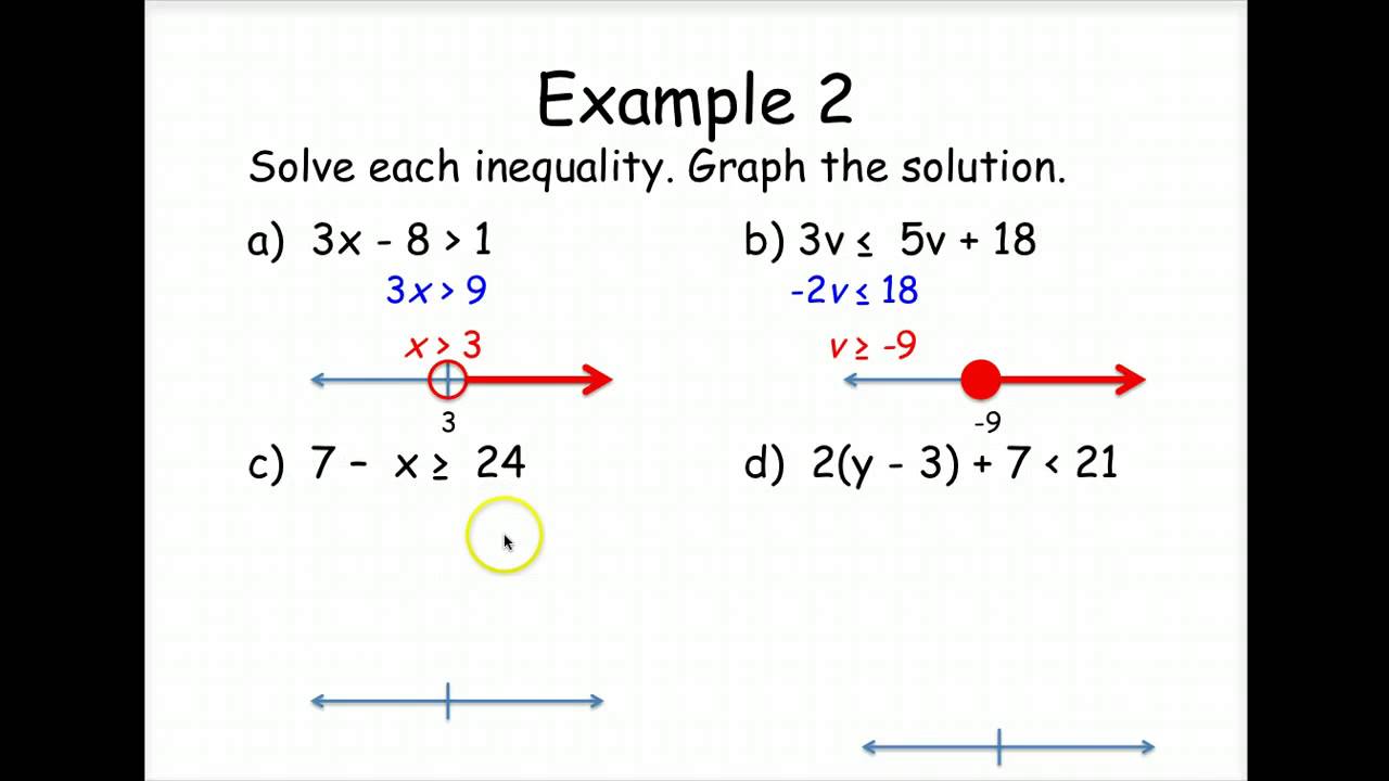
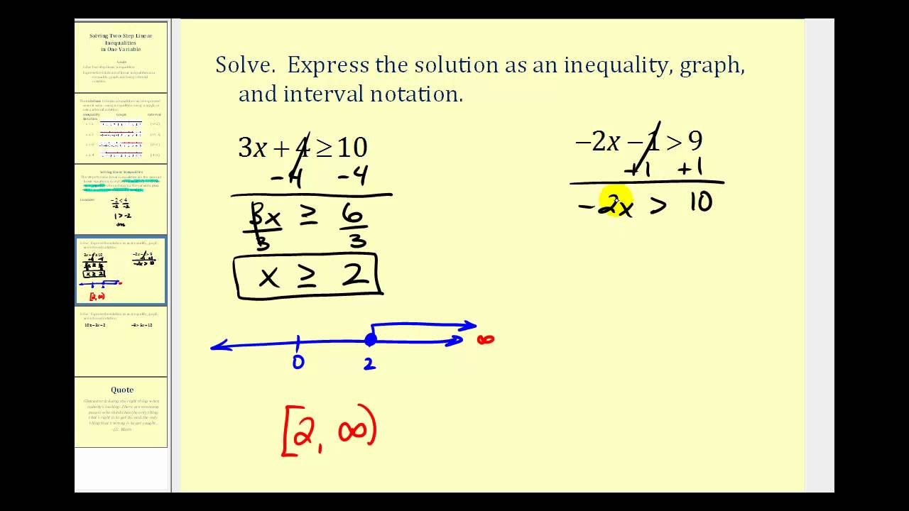
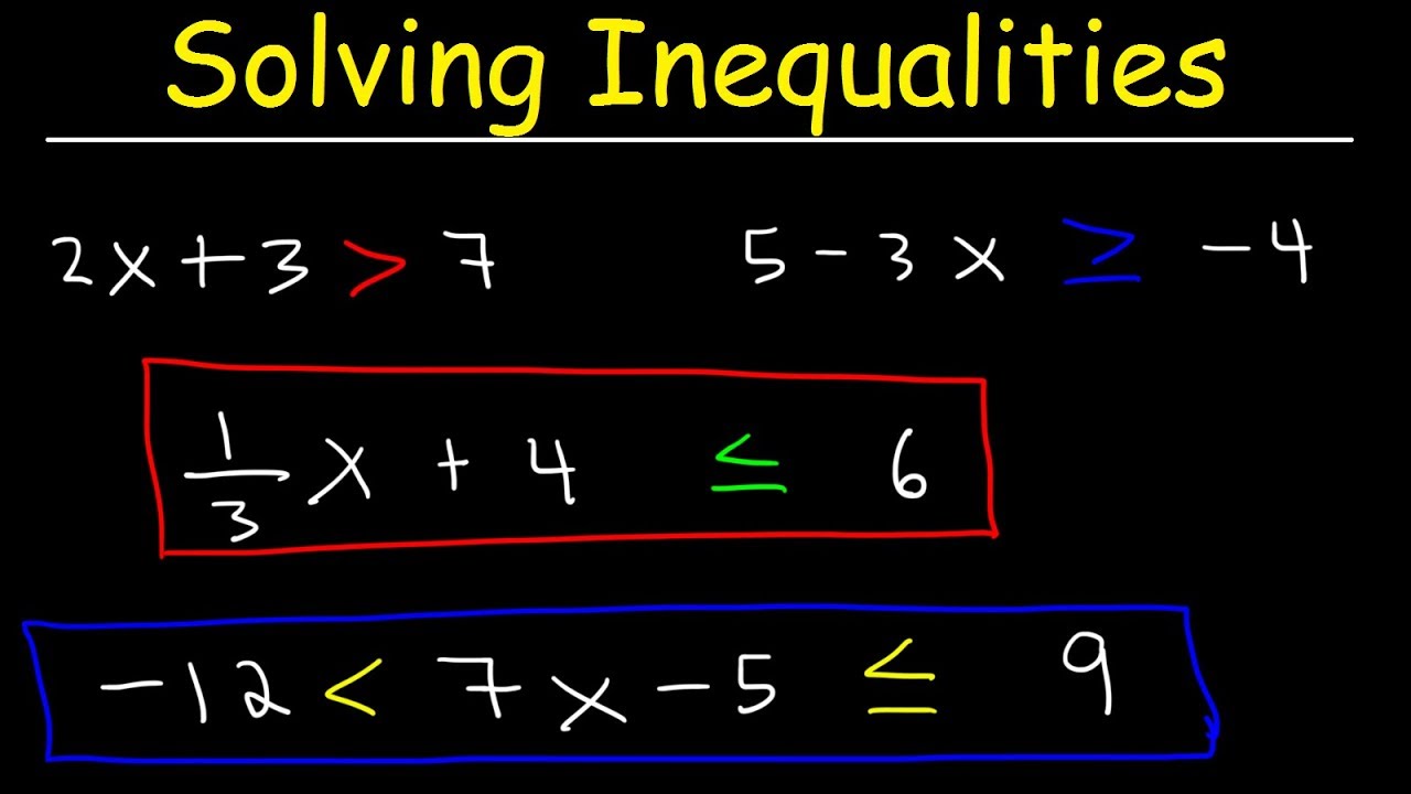
Solving Linear Inequalities

Linear inequalities are similar to linear equations, but they involve comparison operators such as <, >, ≤, or ≥. Solving linear inequalities involves finding the range of values for the variable that satisfies the inequality.To solve linear inequalities, we can use similar methods as for solving linear equations, but with some key differences:* When multiplying or dividing both sides of the inequality by a negative number, we must reverse the inequality sign.

The solution to a linear inequality is typically represented as an interval or a set of values.

For example, to solve the inequality 2x + 3 < 7, we can subtract 3 from both sides, then divide both sides by 2 to get x < 2. This solution represents all values of x that are less than 2.

Graphing Linear Inequalities

Graphing linear inequalities involves shading the region on the coordinate plane that represents the solution set. The boundary line of the shaded region is determined by the corresponding linear equation.To determine which side of the boundary line to shade, we can choose a test point that is not on the line.

If the test point satisfies the inequality, we shade the side containing the test point. Otherwise, we shade the other side.For example, to graph the inequality y > x + 1, we first graph the line y = x + 1.

Then, we choose a test point, such as (0, 0). Since 0 > 0 + 1 is not true, we shade the region above the line.

Systems of Linear Equations

Systems of linear equations are a fundamental concept in algebra that involves finding solutions that satisfy multiple equations simultaneously. These systems are used to represent real-world situations with multiple variables and constraints, enabling us to analyze and solve problems in various fields, including economics, engineering, and physics.

Solving Systems of Equations

There are various methods to solve systems of linear equations, each with its strengths and weaknesses.

• Graphing: This method involves plotting the lines represented by each equation on a coordinate plane. The intersection point of the lines represents the solution that satisfies both equations.
• Substitution: This method involves solving one equation for one variable and substituting it into the other equation.

  This eliminates one variable, resulting in a single equation that can be solved for the remaining variable. The solution can then be substituted back into either original equation to find the value of the other variable.

• Elimination: This method involves manipulating the equations to eliminate one variable by adding or subtracting them.

  This results in a single equation that can be solved for the remaining variable. The solution can then be substituted back into either original equation to find the value of the other variable.

Solving Systems of Inequalities

Systems of inequalities involve finding solutions that satisfy multiple inequalities simultaneously. These systems are represented by a shaded region on a coordinate plane that represents all the points that satisfy all the inequalities.

• Graphing: This method involves graphing the lines represented by each inequality on a coordinate plane. The solution is the region where the shaded areas of all the inequalities overlap.

Examples

Solving a System of Equations by Substitution

Solve the following system of equations:

y = 2x + 1

x + 2y = 11

Substitute the first equation into the second equation:

x + 2(2x + 1) = 11

Simplify and solve for x:

• x + 4x + 2 = 11
• x = 9

x = 9/7

Algebra 1 Honors dives into the world of equations and expressions, building a solid foundation for higher math. You’ll tackle topics like solving linear equations, graphing functions, and working with polynomials. It’s a bit like learning a new language, like Polish, which can be challenging but rewarding.

How difficult is it to learn Polish language ? It depends on your dedication and approach, just like mastering algebra requires practice and persistence. So, while algebra might seem tough, with the right effort, you’ll be solving equations like a pro in no time!

Substitute the value of x back into the first equation to find y:

y = 2(9/7) + 1y = 25/7

Therefore, the solution to the system of equations is (9/7, 25/7).

Solving a System of Inequalities by Graphing

Solve the following system of inequalities:

y > x + 1y < -2x + 3

Graph the lines y = x + 1 and y =

• 2x + 3 on a coordinate plane. The first inequality represents all the points above the line y = x + 1, while the second inequality represents all the points below the line y =
• 2x + 3. The solution is the shaded region where the two shaded areas overlap.

Polynomials

Polynomials are algebraic expressions that consist of variables and coefficients combined using addition, subtraction, and multiplication, where the exponents of the variables are non-negative integers. They are fundamental building blocks in algebra and have applications in various fields like physics, engineering, and economics.

Types of Polynomials

Polynomials can be classified based on the number of terms and the highest degree of the variable.

• Monomial:A polynomial with one term, for example, 3x, 5y², or -7.
• Binomial:A polynomial with two terms, for example, 2x + 5, x² – 4, or 3y³ – 2y.
• Trinomial:A polynomial with three terms, for example, x² + 2x – 1, 4y² – 3y + 2, or 2z³ + 5z – 7.
• Polynomial:A polynomial with more than three terms, for example, x⁴ + 3x³ – 2x² + 5x – 1.

Operations on Polynomials

Polynomials can be added, subtracted, multiplied, and divided, similar to other algebraic expressions.

Addition and Subtraction

To add or subtract polynomials, combine like terms (terms with the same variable and exponent). For example:

(2x² + 3x

• 1) + (x²
• 2x + 5) = 3x² + x + 4

Multiplication

To multiply polynomials, use the distributive property. For example:

(x + 2)(x

• 3) = x(x
• 3) + 2(x
• 3) = x²
• 3x + 2x
• 6 = x²
• x
• 6

Division

Polynomial division is a bit more complex and involves long division or synthetic division. It’s used to divide one polynomial by another. For example, dividing x³ + 2x²5x + 1 by x

1

x² + 3x

• 2 + 1/(x
• 1)

Factoring Polynomials

Factoring polynomials involves expressing a polynomial as a product of simpler polynomials. This is useful for solving polynomial equations.

• Factoring by grouping:This method involves grouping terms with common factors. For example, factoring x³ + 2x² – 5x – 10:

  x²(x + 2)- 5(x + 2) = (x² – 5)(x + 2)

• Factoring using special patterns:Certain polynomials can be factored using specific patterns, such as the difference of squares, sum or difference of cubes, or perfect square trinomials. For example, factoring x² – 9:

  (x + 3)(x- 3)

Solving Polynomial Equations

Polynomial equations are equations where one side is a polynomial expression set equal to zero. To solve them, we can use various methods, including:

• Factoring:Factor the polynomial and set each factor equal to zero. For example, solving x² – 4 = 0:

  (x + 2)(x- 2) = 0 x + 2 = 0 or x – 2 = 0 x = -2 or x = 2

• Quadratic Formula:This formula can be used to solve quadratic equations (polynomials with a degree of 2). For example, solving x² + 2x – 3 = 0:

  x = (-b ± √(b²- 4ac)) / 2a x = (-2 ± √(2² – 4 – 1 – -3)) / 2 – 1 x = (-2 ± √16) / 2 x = (-2 ± 4) / 2 x = 1 or x = -3

Quadratic Equations

Quadratic equations are a fundamental part of algebra, appearing in various applications across science, engineering, and finance. They are equations that involve a variable raised to the second power, along with other terms that may include the variable raised to the first power or a constant term.

Understanding quadratic equations and their properties is crucial for solving problems related to projectile motion, optimization, and other real-world scenarios.

Understanding Quadratic Equations

A quadratic equation is an equation of the form ax² + bx + c = 0, where a, b, and c are constants, and a ≠ 0. The term ax² is the quadratic term, bx is the linear term, and c is the constant term.

The coefficients a, b, and c determine the shape and position of the graph of the quadratic equation, which is a parabola.Here are some examples of quadratic equations:

• 2x² + 5x
• 3 = 0
• x²
• 4 = 0
• 3x² + 2x = 0

In the first example, a = 2, b = 5, and c =

• 3. In the second example, a = 1, b = 0, and c =
• 4. In the third example, a = 3, b = 2, and c = 0.

Methods for Solving Quadratic Equations

Solving a quadratic equation means finding the values of x that satisfy the equation. There are several methods for solving quadratic equations, each with its own advantages and disadvantages.

Factoring Quadratic Equations

Factoring is a method of solving quadratic equations by expressing the quadratic expression as a product of two linear factors. This method relies on recognizing common factoring patterns and applying the distributive property.Here are the steps involved in factoring a quadratic equation:

1. Factor out the greatest common factor (GCF)

If there is a common factor among all the terms, factor it out.

2. Factor the remaining expression

Factor the remaining expression into two linear factors.

3. Set each factor equal to zero

Set each linear factor equal to zero and solve for x.Here are some examples of factoring quadratic equations:

Example 1

x² + 5x + 6 = 0

(x + 2)(x + 3) = 0

x + 2 = 0 or x + 3 = 0

• x =
• 2 or x =
• 3

Example 2

• 2x²
• 5x
• 3 = 0

• (2x + 1)(x
• 3) = 0

• 2x + 1 = 0 or x
• 3 = 0

• x =
• 1/2 or x = 3

Completing the Square

Completing the square is a method of solving quadratic equations by manipulating the equation to form a perfect square trinomial. This method is particularly useful when factoring is not readily apparent or when dealing with equations that have fractional coefficients.Here are the steps involved in completing the square:

1. Move the constant term to the right side of the equation

This isolates the x² and x terms on the left side.

2. Divide both sides of the equation by the coefficient of x²

This ensures that the coefficient of x² is 3. Take half of the coefficient of x, square it, and add it to both sides of the equation:This creates a perfect square trinomial on the left side.

4. Factor the perfect square trinomial

The left side can now be factored as (x + h)², where h is half of the coefficient of x.

5. Solve for x

Take the square root of both sides and solve for x.Here is an example of completing the square:

Example

• x² + 6x
• 7 = 0

x² + 6x = 7

x² + 6x + 9 = 7 + 9

(x + 3)² = 16

x + 3 = ±4

• x =
• 3 ± 4

• x = 1 or x =
• 7

The Quadratic Formula

The quadratic formula is a general solution for quadratic equations, providing a direct way to find the roots of any quadratic equation. It is derived by completing the square on the general quadratic equation ax² + bx + c = 0.The quadratic formula is:

x = (-b ± √(b²

4ac)) / 2a

where a, b, and c are the coefficients of the quadratic equation.The discriminant (b²

4ac) determines the nature of the roots

• If the discriminant is positive, the quadratic equation has two distinct real roots.
• If the discriminant is zero, the quadratic equation has one real root (a double root).
• If the discriminant is negative, the quadratic equation has two complex roots.

Here are some examples of using the quadratic formula:

Example 1

• x²
• 5x + 6 = 0

• a = 1, b =
• 5, c = 6

• x = (5 ± √((-5)²
• 4
• 1
• 6)) / (2
• 1)

x = (5 ± √1) / 2

x = 3 or x = 2

Example 2

2x² + 4x + 2 = 0

a = 2, b = 4, c = 2

• x = (-4 ± √(4²
• 4
• 2
• 2)) / (2
• 2)

x = (-4 ± √0) / 4

• x =
• 1

Graphing Quadratic Functions

A quadratic function is a function of the form y = ax² + bx + c, where a, b, and c are constants and a ≠ 0. The graph of a quadratic function is a parabola, which is a symmetrical U-shaped curve.The key features of a quadratic function and its graph include:

Vertex

The vertex is the lowest or highest point on the parabola, depending on the sign of the coefficient ‘a’. The coordinates of the vertex can be found using the formula (-b/2a, f(-b/2a)).

Axis of Symmetry

The axis of symmetry is a vertical line that passes through the vertex and divides the parabola into two symmetrical halves. The equation of the axis of symmetry is x =b/2a.

Y-intercept

The y-intercept is the point where the parabola intersects the y-axis. It can be found by setting x = 0 in the equation of the quadratic function.

Concavity

The concavity of the parabola is determined by the sign of the coefficient ‘a’. If ‘a’ is positive, the parabola opens upward (concave up). If ‘a’ is negative, the parabola opens downward (concave down).Here are the steps involved in graphing a quadratic function:

1. Find the vertex

Use the formula (-b/2a, f(-b/2a)) to find the coordinates of the vertex.

2. Find the axis of symmetry

The axis of symmetry is the vertical line x =b/2a.

• 3. Find the y-intercept

  Set x = 0 in the equation of the quadratic function to find the y-intercept.

• Plot the vertex, axis of symmetry, and y-intercept:Plot these points on a coordinate plane.

5. Choose additional points

Choose a few more x-values on either side of the vertex and calculate the corresponding y-values. Plot these points on the coordinate plane.

6. Draw the parabola

Connect the plotted points with a smooth curve to form the parabola.

Here is an example of graphing a quadratic function:

Example

• y = x²
• 4x + 3

Vertex

(-b/2a, f(-b/2a)) = (2,

1)

Axis of symmetry

x = 2

Y-intercept

(0, 3)

Plot these points on a coordinate plane and choose additional points to draw the parabola.

The solutions (roots) of a quadratic equation correspond to the x-intercepts of the graph of the corresponding quadratic function. These are the points where the parabola intersects the x-axis.

7. Functions and Their Graphs

Functions are a fundamental concept in algebra and mathematics, representing a special relationship between input and output values. Understanding functions allows us to model and analyze real-world phenomena, from the growth of a population to the trajectory of a projectile.

7.1 Understanding Functions

A function is a rule that assigns exactly one output value to each input value. The input value is called the domain, and the output value is called the range. The relationship between input and output is often represented by an equation, where the input variable is typically denoted by

• x* and the output variable by
• y*.

• Linear Functions:Linear functions have a constant rate of change, resulting in a straight line when graphed. They are represented by equations of the form -y = mx + b*, where -m* is the slope and -b* is the y-intercept. For example, the function -y = 2x + 1* represents a linear function with a slope of 2 and a y-intercept of 1.

• Quadratic Functions:Quadratic functions have a variable rate of change, resulting in a parabolic curve when graphed. They are represented by equations of the form -y = ax^2 + bx + c*, where -a*, -b*, and -c* are constants. For example, the function -y = x^2 – 4x + 3* represents a quadratic function with a vertex at (2, -1).

• Exponential Functions:Exponential functions exhibit rapid growth or decay, characterized by a constant multiplicative factor. They are represented by equations of the form -y = ab^x*, where -a* is the initial value and -b* is the growth factor. For example, the function -y = 2^x* represents an exponential function with a growth factor of 2.

• Trigonometric Functions:Trigonometric functions relate the angles of a right triangle to the lengths of its sides. They are used to model periodic phenomena, such as sound waves and the movement of a pendulum. Examples include sine (sin), cosine (cos), and tangent (tan).

7.2 Domain and Range

The domainof a function is the set of all possible input values. The rangeof a function is the set of all possible output values.

• To determine the domain of a function, we look for any restrictions on the input values. For example, the function -y = 1/x* has a domain of all real numbers except for -x = 0*, because division by zero is undefined.

• To determine the range of a function, we look at the possible output values. For example, the function -y = x^2* has a range of all non-negative real numbers, because the square of any real number is always non-negative.

7.3 Graphical Representation

The graph of a function is a visual representation of the relationship between its input and output values. Each point on the graph represents a specific input-output pair.

• To graph a function, we plot points that correspond to input-output pairs. For example, to graph the function -y = x + 2*, we could plot the points (0, 2), (1, 3), and (-1, 1). Connecting these points with a straight line results in the graph of the function.

• The equation of a function provides information about its graph. For example, the slope of a linear function is represented by the coefficient of -x* in its equation. The y-intercept of a linear function is represented by the constant term in its equation.

• Key features of a graph can be identified and interpreted. For example, the x-interceptsof a graph represent the input values where the function equals zero. The y-interceptrepresents the output value when the input is zero. The slopeof a linear function represents the rate of change of the output value with respect to the input value.

7.4 Analyzing and Interpreting Graphs

Graphs of functions are powerful tools for analyzing and interpreting relationships between variables.

• Real-world scenarios can be modeled using functions. For example, the relationship between the number of hours worked and the amount of money earned can be modeled by a linear function. The graph of this function can be used to determine the amount of money earned for a specific number of hours worked, or to determine the number of hours needed to earn a specific amount of money.

• The graph of a function can be used to solve problems. For example, the graph of a quadratic function can be used to find the maximum or minimum value of the function, or to find the input values that correspond to a specific output value.

8. Exponential and Logarithmic Functions

Exponential and logarithmic functions are fundamental concepts in algebra that describe relationships involving growth and decay. They have wide-ranging applications in various fields, including finance, science, and engineering. This section will delve into the properties, applications, and methods for solving equations involving these functions.

Exponential Functions

Exponential functions are used to model situations where a quantity increases or decreases at a constant rate over time. The general form of an exponential function is f(x) = a^x, where ‘a’ is the base and ‘x’ is the exponent.

The base ‘a’ determines the rate of growth or decay, while the exponent ‘x’ represents the time or the number of times the base is multiplied by itself.

• If the base ‘a’ is greater than 1, the function represents exponential growth. As the value of ‘x’ increases, the function grows rapidly.
• If the base ‘a’ is between 0 and 1, the function represents exponential decay. As the value of ‘x’ increases, the function decreases rapidly.
• The graph of an exponential function is a curve that either rises or falls rapidly, depending on the base. The curve never touches the x-axis, but it approaches the x-axis as ‘x’ approaches negative infinity for growth functions and positive infinity for decay functions.

For example, consider the population growth of bacteria. If a colony of bacteria doubles in size every hour, the population can be modeled using an exponential function. The initial population is the base ‘a’, and the time in hours is the exponent ‘x’.

The function would be f(x) = a

2^x, where ‘f(x)’ represents the population after ‘x’ hours.

Applications of Exponential Functions

Exponential functions are widely used in various applications, including:

• Finance: Compound interest calculations, where the interest earned is added to the principal amount, resulting in exponential growth. For example, if you invest $1000 at an annual interest rate of 5%, compounded annually, the amount after ‘x’ years can be calculated using the formula A = 1000 – (1 + 0.05)^x.

• Population growth and decay: Modeling the growth of populations, radioactive decay, and other phenomena that exhibit exponential behavior.
• Physics, chemistry, and biology: Modeling the spread of diseases, the decay of radioactive materials, and the growth of organisms.

Logarithmic Functions

Logarithmic functions are the inverses of exponential functions. They are used to solve for the exponent in an exponential equation. The general form of a logarithmic function is log_a(x) = y, which is equivalent to a^y = x. In this notation, ‘a’ is the base of the logarithm, ‘x’ is the argument, and ‘y’ is the logarithm.

• The base ‘a’ of the logarithm is the same as the base of the corresponding exponential function.
• The graph of a logarithmic function is a curve that rises or falls slowly, depending on the base. The curve never touches the y-axis, but it approaches the y-axis as ‘x’ approaches zero.

For example, if you want to find the time it takes for a certain amount of money to double at a given interest rate, you can use a logarithmic function. The amount of money is the argument ‘x’, the interest rate is the base ‘a’, and the time is the logarithm ‘y’.

Relationship between Exponential and Logarithmic Functions

Exponential and logarithmic functions are intimately related. They are inverse functions of each other, meaning that they undo each other’s operations. This relationship is crucial for solving equations involving exponential and logarithmic functions.

• Logarithmic functions can be used to solve exponential equations by converting the exponential equation into a logarithmic equation.
• The properties of logarithms, such as the product rule, quotient rule, and power rule, can be used to simplify logarithmic expressions.
• Exponential and logarithmic forms can be interchanged using the following rules:
  • If a^y = x, then log_a(x) = y.
  • If log_a(x) = y, then a^y = x.

For example, consider the equation 2^x = 8. To solve for ‘x’, we can take the logarithm of both sides with base 2. This gives us log_2(2^x) = log_2(8). Using the property that log_a(a^x) = x, we get x = log_2(8).

Since 2^3 = 8, we know that log_2(8) = 3. Therefore, the solution to the equation 2^x = 8 is x = 3.

9. Sequences and Series: What Do You Learn In Algebra 1 Honors

Sequences and series are fundamental concepts in mathematics that deal with ordered lists of numbers. They are widely used in various fields, including finance, physics, and computer science. In this section, we will explore the different types of sequences and series, their properties, and their applications.

Introduction to Sequences and Series

A sequence is an ordered list of numbers, where each number is called a term. A series is the sum of the terms of a sequence. Sequences and series can be either finite or infinite. A finite sequence or series has a limited number of terms, while an infinite sequence or series has an unlimited number of terms.Here are some real-world examples of sequences and series:

Compound Interest

The amount of money in a savings account after each compounding period forms a geometric sequence.

Population Growth

The population of a city over time can be modeled using an arithmetic or geometric sequence.

Fibonacci Sequence

This sequence, where each term is the sum of the two preceding terms (e.g., 1, 1, 2, 3, 5, 8), appears in various natural phenomena, such as the arrangement of leaves on a stem and the spiral patterns of seashells.

Arithmetic Sequences

An arithmetic sequence is a sequence where the difference between any two consecutive terms is constant. This constant difference is called the common difference.The nth term of an arithmetic sequence can be found using the formula:

a_n= a ₁+ (n

1)d

where:

• a _nis the nth term
• a ₁is the first term
• d is the common difference
• n is the number of terms

For example, the sequence 2, 5, 8, 11, 14… is an arithmetic sequence with a common difference of 3. The 5th term of this sequence is a ₅= 2 + (5

1)3 = 14.

Geometric Sequences

A geometric sequence is a sequence where the ratio between any two consecutive terms is constant. This constant ratio is called the common ratio.The nth term of a geometric sequence can be found using the formula:

a_n= a ₁

• r ⁽ⁿ
• 1)

where:

• a _nis the nth term
• a ₁is the first term
• r is the common ratio
• n is the number of terms

For example, the sequence 3, 6, 12, 24, 48… is a geometric sequence with a common ratio of 2. The 5th term of this sequence is a ₅= 3

• 2 ⁽⁵
• 1)= 48.

Sum of Finite Arithmetic Series

The sum of a finite arithmetic series is the sum of the terms of an arithmetic sequence. The formula for the sum of a finite arithmetic series is:

S_n= (n/2)(a ₁+ a _n)

where:

• S _nis the sum of the first n terms
• a ₁is the first term
• a _nis the nth term
• n is the number of terms

For example, the sum of the first 5 terms of the arithmetic sequence 2, 5, 8, 11, 14 is S ₅= (5/2)(2 + 14) = 40.

Sum of Finite Geometric Series

The sum of a finite geometric series is the sum of the terms of a geometric sequence. The formula for the sum of a finite geometric series is:

S_n= a ₁(1

• r ⁿ) / (1
• r)

where:

• S _nis the sum of the first n terms
• a ₁is the first term
• r is the common ratio
• n is the number of terms

For example, the sum of the first 5 terms of the geometric sequence 3, 6, 12, 24, 48 is S ₅= 3(1

• 2 ⁵) / (1
• 2) = 93.

Sum of Infinite Geometric Series

An infinite geometric series converges if the absolute value of the common ratio is less than 1 (|r| < 1). The formula for the sum of a convergent infinite geometric series is:

S_∞= a ₁/ (1

r)

where:

• S _∞is the sum of the infinite series
• a ₁is the first term
• r is the common ratio

For example, the infinite geometric series 1 + 1/2 + 1/4 + 1/8 + … has a common ratio of 1/2, which is less than 1. Therefore, the series converges, and its sum is S _∞= 1 / (1

1/2) = 2.

Applications of Sequences and Series

Sequences and series have numerous applications in various fields, including:

Compound Interest

The formula for compound interest involves a geometric series.

Population Growth

Population models often use arithmetic or geometric sequences to predict future population sizes.

Annuities

Annuities, which are a series of regular payments, can be calculated using geometric series.

Patterns in Nature

Sequences and series appear in various natural phenomena, such as the Fibonacci sequence in plant growth and the arrangement of petals in a flower.

Data Analysis and Statistics

Data analysis is a crucial aspect of algebra, allowing us to extract meaningful insights from raw data. It involves organizing, summarizing, and interpreting data to identify patterns, trends, and relationships. Understanding data analysis equips us with the tools to make informed decisions and solve real-world problems.

Measures of Central Tendency

Measures of central tendency provide a single value that represents the typical or average value in a dataset. They help us understand the center of the data distribution.

• Mean:The sum of all values divided by the total number of values. It is the most commonly used measure of central tendency.
• Median:The middle value in a sorted dataset. It is less affected by outliers than the mean.
• Mode:The value that appears most frequently in a dataset. There can be multiple modes or no mode.

Measures of Dispersion

Measures of dispersion describe the spread or variability of data points around the central tendency. They tell us how much the data values differ from each other.

• Range:The difference between the highest and lowest values in a dataset. It provides a simple measure of the spread but is sensitive to outliers.
• Variance:The average squared deviation of each data point from the mean. It measures how much the data values vary around the mean.
• Standard Deviation:The square root of the variance. It provides a more interpretable measure of spread than variance, as it is in the same units as the original data.

Interpreting and Analyzing Data

Statistical methods enable us to interpret and analyze data effectively. By calculating measures of central tendency and dispersion, we can gain a deeper understanding of the data’s characteristics and draw meaningful conclusions.

For example, consider a dataset of student test scores. The mean score might represent the average performance of the class. The standard deviation would indicate the spread of scores around the average. A high standard deviation suggests a wide range of scores, while a low standard deviation suggests scores are clustered around the mean.

11. Applications of Algebra

Algebra is not just a subject you learn in school; it’s a powerful tool that has applications in various fields, shaping the world around us. From understanding the laws of nature to designing complex structures and managing finances, algebra plays a crucial role in solving real-world problems.

Science

Algebra is a fundamental tool in various scientific disciplines, providing a framework for modeling and analyzing natural phenomena.

• Physics:Algebra is used extensively in physics to model motion, forces, and energy. For example, the equation d = vt, where drepresents distance, vrepresents velocity, and trepresents time, is used to calculate the distance traveled by an object moving at a constant velocity.

  Another example is the equation F = ma, where Frepresents force, mrepresents mass, and arepresents acceleration, which describes the relationship between force, mass, and acceleration. This equation is crucial for understanding how objects move and interact with each other.

• Chemistry:In chemistry, algebra is essential for stoichiometry calculations, which involve determining the quantities of reactants and products in chemical reactions. For instance, balancing chemical equations requires using algebraic equations to ensure that the number of atoms of each element on both sides of the equation is equal.

  For example, the balanced chemical equation for the reaction of hydrogen gas (H ₂) with oxygen gas (O ₂) to form water (H ₂O) is: 2H ₂+ O ₂→ 2H ₂O. Algebra helps ensure that the number of hydrogen and oxygen atoms on both sides of the equation are equal.

• Biology:Algebra is applied in population dynamics to model how populations of organisms grow and change over time. For example, the logistic growth model, which describes the growth of a population with limited resources, uses algebraic equations to predict population size.

  Algebra is also used in genetic analysis to understand how genes are passed from parents to offspring and to predict the likelihood of certain traits appearing in future generations.

Engineering

Algebra is a fundamental tool in various engineering disciplines, providing a framework for designing, analyzing, and building structures and systems.

• Civil Engineering:In civil engineering, algebra is used in structural analysis to calculate the forces and stresses on buildings, bridges, and other structures. Engineers use algebraic equations to determine the load-bearing capacity of structures and ensure their stability. For example, the equation σ = F/A, where σrepresents stress, Frepresents force, and Arepresents area, is used to calculate the stress on a material under a given load.

  This equation helps engineers design structures that can withstand the expected forces and stresses.

• Electrical Engineering:Electrical engineers use algebra in circuit analysis to calculate current, voltage, and resistance in electrical circuits. The equation V = IR, where Vrepresents voltage, Irepresents current, and Rrepresents resistance, is a fundamental equation in electrical engineering. This equation helps engineers design and analyze electrical circuits and systems.

• Mechanical Engineering:Mechanical engineers use algebra in kinematics and dynamics to analyze the motion and forces of moving objects. For example, the equation v = u + at, where vrepresents final velocity, urepresents initial velocity, arepresents acceleration, and trepresents time, is used to calculate the final velocity of an object undergoing constant acceleration.

  This equation helps engineers design machines and systems that operate efficiently and safely.

Finance

Algebra is a vital tool in finance, enabling individuals and businesses to make informed financial decisions.

• Personal Finance:In personal finance, algebra is used in budgeting to track income and expenses, calculate loan payments, and analyze investment returns. For example, the equation A = P(1 + r/n)^nt, where Arepresents the future value of an investment, Prepresents the principal amount, rrepresents the interest rate, nrepresents the number of times interest is compounded per year, and trepresents the time period in years, is used to calculate the future value of an investment.

  This equation helps individuals plan for their financial future.

• Business Finance:Business finance professionals use algebra in financial modeling to forecast future financial performance, assess risk, and make investment decisions. For example, the equation NPV =-C ₀+ Σ _t=1ⁿCF _t/(1+r) ^t, where NPVrepresents the net present value of an investment, C₀represents the initial investment cost, CF_trepresents the cash flow in period t, rrepresents the discount rate, and nrepresents the number of periods, is used to calculate the net present value of an investment.

  This equation helps businesses evaluate the profitability of different investment opportunities.

Problem-Solving and Critical Thinking

Algebra equips individuals with essential problem-solving and critical thinking skills, enabling them to approach complex situations with logic and reason.

• Breaking Down Complex Problems:Algebra teaches students how to break down complex problems into smaller, manageable steps. By representing relationships with variables and equations, students can analyze each step systematically and arrive at a solution.
• Critical Thinking:Algebra emphasizes critical thinking, including analyzing information, identifying patterns, and making logical deductions. Students learn to interpret data, formulate hypotheses, and draw conclusions based on evidence.
• Real-World Applications:The problem-solving and critical thinking skills developed in algebra are valuable in various real-world scenarios. For example, a scientist might use algebra to analyze experimental data, an engineer might use algebra to design a bridge, or a financial analyst might use algebra to model market trends.

Problem-Solving Strategies

Algebra is more than just manipulating equations; it’s a powerful tool for solving real-world problems. Mastering problem-solving strategies is crucial for applying algebraic concepts effectively.

Understanding the Problem

Before diving into calculations, it’s essential to understand the problem’s context. Read the problem carefully, identify the unknown quantities, and determine what information is given. Visualizing the problem with a diagram or table can be helpful.

Formulating Equations

Once you understand the problem, translate the information into mathematical equations. Look for key words that indicate mathematical operations. For example, “sum” suggests addition, “difference” suggests subtraction, “product” suggests multiplication, and “quotient” suggests division.

Solving Equations

Use the appropriate algebraic techniques to solve the equations you’ve formulated. This might involve simplifying expressions, isolating variables, or using various algebraic properties.

Checking Your Solution

After finding a solution, always check if it makes sense in the context of the original problem. Substitute the solution back into the original equations or the problem’s description to ensure it satisfies all conditions.

Example

Let’s say you want to find the length and width of a rectangular garden whose perimeter is 30 meters and whose length is 2 meters more than its width. First, identify the unknowns:

• Length (l)
• Width (w)

Next, translate the information into equations:

Perimeter

2l + 2w = 30

Length is 2 meters more than width

l = w + 2Now, substitute the second equation into the first equation:

2(w + 2) + 2w = 30

Solve for w:

• 2w + 4 + 2w = 30
• 4w + 4 = 30
• 4w = 26
• w = 6.5 meters

Substitute w back into the equation for l:

• l = 6.5 + 2
• l = 8.5 meters

Therefore, the length of the garden is 8.5 meters and the width is 6.5 meters.

13. Advanced Topics in Algebra

Algebra 1 Honors provides a strong foundation in fundamental algebraic concepts. However, venturing into advanced topics like matrices, vectors, and trigonometry unveils a deeper understanding of mathematics and its applications in various fields. These topics build upon the knowledge acquired in Algebra 1 Honors, expanding your mathematical toolkit and preparing you for more complex mathematical explorations.

Matrices

Matrices are rectangular arrays of numbers, symbols, or expressions arranged in rows and columns. They are a powerful tool for representing and manipulating data, especially in systems of equations, linear transformations, and computer graphics.Matrices can be added, subtracted, and multiplied, with specific rules governing these operations.

Matrix addition and subtraction involve adding or subtracting corresponding elements of two matrices of the same dimensions.

Matrix multiplication, however, involves a more complex process that combines elements from rows of the first matrix with elements from columns of the second matrix.

Matrices can represent systems of linear equations efficiently. Each row of the matrix corresponds to an equation, and each column represents a variable.

For example, the system of equations:

x + 3y = 7

x

2y = 1

can be represented by the matrix:[ 2 3 ] [ x ] = [ 7 ][ 1

2 ] [ y ] [ 1 ]

Matrix inverses play a crucial role in solving systems of equations. The inverse of a matrix, denoted by A ^-1, is a matrix that, when multiplied by the original matrix A, results in the identity matrix.

The identity matrix is a square matrix with 1s on the diagonal and 0s elsewhere.

By multiplying both sides of the matrix equation representing a system of equations by the inverse of the coefficient matrix, we can isolate the variables and solve the system.

Vectors

Vectors are mathematical objects that have both magnitude (length) and direction. They are often represented by arrows, where the length of the arrow represents the magnitude and the direction of the arrow indicates the vector’s direction.Vectors can be added, subtracted, and multiplied by scalars (numbers).

Vector addition involves placing the tail of one vector at the head of the other and drawing the resultant vector from the tail of the first vector to the head of the second vector.

Vector subtraction is similar to addition, but involves adding the negative of the second vector to the first vector.

Scalar multiplication involves multiplying each component of a vector by the scalar.

The dot product of two vectors is a scalar quantity that measures the projection of one vector onto the other.

The dot product of vectors a and b is calculated as: a · b = |a| |b| cos θ, where θ is the angle between the two vectors.

The cross product of two vectors is a vector quantity that is perpendicular to both of the original vectors.

The cross product of vectors a and b is calculated as: a × b = |a| |b| sin θ n, where θ is the angle between the two vectors and n is a unit vector perpendicular to both a and b.

Vectors have numerous applications in physics, engineering, and computer graphics. For example, they are used to represent forces, velocities, and displacements.

Trigonometry

Trigonometry deals with the relationships between the sides and angles of triangles. The basic trigonometric functions are sine, cosine, and tangent.

The sine of an angle is defined as the ratio of the opposite side to the hypotenuse.

The cosine of an angle is defined as the ratio of the adjacent side to the hypotenuse.

The tangent of an angle is defined as the ratio of the opposite side to the adjacent side.

The unit circle is a circle with a radius of 1 centered at the origin of a coordinate plane. It is used to visualize and understand trigonometric functions for all angles.The laws of sines and cosines are used to solve triangles when not all sides and angles are known.

The law of sines states that the ratio of the sine of an angle to the length of the opposite side is constant for all angles in a triangle.

The law of cosines states that the square of one side of a triangle is equal to the sum of the squares of the other two sides minus twice the product of those sides and the cosine of the included angle.

Trigonometry has numerous applications in surveying, navigation, and physics.

Building upon Algebra 1 Honors

Matrices, vectors, and trigonometry build upon the foundations of Algebra 1 Honors in several ways.Matrices provide a powerful tool for solving systems of linear equations, which is a key topic in Algebra 1 Honors.Vectors are closely related to the concept of functions, as they can be used to represent points in space and to define transformations.Trigonometry builds upon the concept of angles and their relationships to sides of triangles, which is introduced in geometry.The advanced topics in algebra provide a deeper understanding of the mathematical concepts learned in Algebra 1 Honors and open up new avenues for exploring and applying mathematics in various fields.

FAQ Resource

What are the prerequisites for Algebra 1 Honors?

Typically, a strong foundation in pre-algebra and a solid understanding of basic mathematical concepts are required. You should also have a strong work ethic and a willingness to challenge yourself.

Is Algebra 1 Honors harder than regular Algebra 1?

Yes, Algebra 1 Honors is generally considered more challenging due to its faster pace, deeper coverage of topics, and higher expectations for problem-solving and critical thinking.

What are some tips for succeeding in Algebra 1 Honors?

Stay organized, attend class regularly, participate actively, seek help when needed, and practice regularly. Don’t be afraid to ask questions and work with your classmates.

What are some career paths that benefit from Algebra 1 Honors?

Fields like engineering, computer science, medicine, finance, and research often require strong math skills, making Algebra 1 Honors a valuable foundation for these career paths.